Target audience: Absolute beginners trying to understand Convolutional neural nets intuitively

Not too long ago, I used to claim to do “Deep Learning” (air-quotes) by building image classifiers.

Most of the classifiers I’d built up to until this point was mostly by running transfer learning on the once-upon-a-time-state-of-the-art InceptionV3. But that was before I joined Fynd. Once I came here, it exposed me to real-world applications of deep learning which most often extended beyond classic classifiers.

With the goal of wanting to move to the research domain, I planned to become TensorFlow certified

Thanks to Google’s suggestions, I came across this YouTube video about how this guy got TensorFlow certified.

From this I came across the TensorFlow in Practise Specialisation from Coursera.

With all the resources under my belt, I decided to actually learn how to build custom models and this time, unlike always understand what was happening under the hood.

To my surprise, the Keras API is actually very easy to use once you’re familiar with what you’re doing.

Anyway, without much further, lets get started (insert finger-snap and transformers sound like JerryRigEverything).

What are convolutions?

So in super simple words, convolutions were devised to capture the spatial information of an image. It preserves the essence of the image but reduces the dimensionality significantly.

Convolutions consist of something called a filter which is usually pre-defined for whatever we’re trying to highlight.

You’re probably wonder, what on earth is a filter, what highlight?

Well, clearly these are textbook definitions, lets take a deep dive into what all that gibberish actually means.

Understanding convolutions

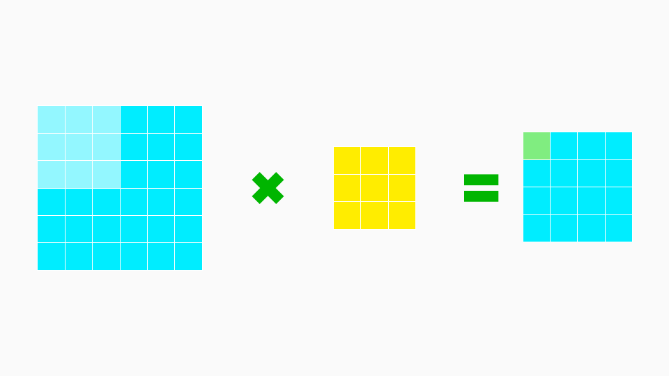
Here’s the convolution GIF that every blog usually tends to include

You might be wondering

But what’s really happening in this “sliding window”?

How are these green squares on the right being generated?

To understand this, we’ll need to understand what does the blue and yellow blocks mean. Lets break it down into more simpler terms that will make it easier to understand.

Blue “Box”

The blue grid on the left is the image input. This can be of NxM dimensions but for ease of understanding, lets take a simple image with 6x6px dimensions.

Yellow “Box”

The yellow box is whats called the filter.

There are many types of filters and all they really do is highlight specific features and remove the other features. Images tend to have vertical lines, horizontal lines, curves that join together to make up the image.

Green “Box”

Each single green box is the output of the calculation done when a filter is placed on the image. I’ll explain more in detail how this calculation occurs.

Finding the value of Green “Box”

It might look complex but trust me, its super simple. This is coming from someone who has flunk a Math exam in his postgrad and hasn’t done formal training in maths during high-school. You will however need to be familiar with how matrix additions/multiplications work and how x and y coordinates can be used to traverse in a 2d plane.

To understand the whole process, lets just take step one and dissect the calculations

We’ll make a calculation of what happens in this one single step, which is shown in the image below.

The light blue part on the left image, is the place where we impose or place our filter(yellow boxes).

When that’s happening, we can ignore the other pixels 27 pixels(darker blue in the image) as they are not being considered at the moment.

Let’s throw those out of the window(to make it more simple to understand), after which this is what it would look like.

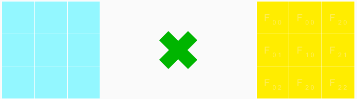
If you noticed that the operator has changed, that’s because we’re now looking at the actual mathematical operator that will be applied in this case.

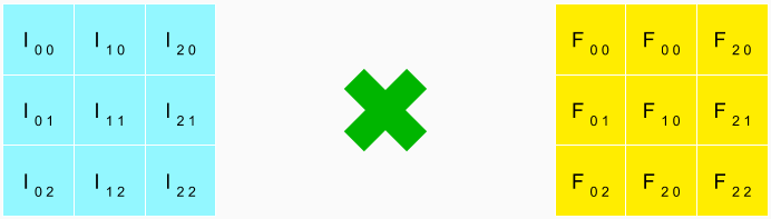
Now for making our life easier, lets give each block an address so that defining it as a formula becomes easier.

Addressing pixels

Lets set the address for these coloured blocks so that we can make it easy to denote it with mathematical notations.

• Image pixels can be denoted as as i x y where i stands for image , x for the x-axis coordinate and y for the y-axis coordinate.
• Filter can be denoted as f x y where f stands for filter, xand y same as above (denoting its address at its own axis)

Here’s what the above image would look like with its addresses.

Calculation of a convolution

In simple words, all we’re doing is multiplying top left pixel of the image with the corresponding top left value of the filter. Next we would do the same for top middle pixel of the image and multiply it with the corresponding top middle value of the filter.

Here’s what the mathematical notation for it would look like:

$$ GREEN_PIXEL = I_{00}*F_{00} + I_{01}*F_{01} + I_{02}*F_{02} + I_{10}*F_{10} + I_{11}*F_{11} + I_{12}*F_{12} + I_{20}*F_{20} + I_{21}*F_{21} + I_{22}*F_{22} $$

Dimensions changed after Convolutions

Now if you guys noticed, in the original step:

We had an image of the dimension: 6x6

But the output was 4x4.

Ideally we should run our filters from the first pixel, but since our filter works on a concept called nearest neighbour, we must pad the Image and the first pixel on which the convolution is actually targetting is I 1 1 and not I 0 0.

Since we can’t run a convolution on neighbours of I 0 0 since no neighbours exist towards the upper and left side of the center, images are usually padded to overcome this.

But since most often edges don’t contain much information we can skip these pixels and calculate the convolutional value for pixels that do have neighbours.

Note: The number of pixels that get skipped/dimension change depends entirely on the window size of the filter sliding around.

Bear in mind, for a filter of 3x3 we would one row and column of pixels each. For a filter of 5x5, we would lose two rows and columns worth of pixel data from the image.

Last modified on 2020-12-22